Topographic and tectonic stress inversions with halfspace: Calculating the topographic stress field
Richard Styron
edited 22 Feb 2015: Equations \(G_{xx}^B\) and \(G_{yy}^B\) corrected
Background of the topographic stress field calculations
The weight of mountains (or other high topography) induces stresses in the earth below the topography. Unlike many other types of stress in the crust, topographic stresses are expected to have very significant spatial variation. Therefore, in regions with high topography, it is important to include topographic stresses into the overall stress budgets of the regions.
But because of this spatial variation in topographic stresses, calculating them is not as straightforward as for some other stress components (such as lithostatic stress, which is basically \(\rho g z\)). As explained in the introduction, we use some techniques based on treating the earth as an elastic halfspace to calculate the stresses. Elastic halfspaces do a good job of representing appropriate (time-invariant) stresses and strains in the earth due to forcing of various sorts. They also typically have simple and well-defined solutions for how the stresses and strains from simple, well-defined perturbations (i.e. other stresses and strains) propagate throughout the halfspace.
When we calculate stresses with halfspace, we use a set of these solutions
relating how a point load (force) of some known magnitude on the surface of the
halfspace induces stresses throughout the halfspace. First, we approximate
topography as a regularly-spaced array of vertical point loads
(the Digital Elevation Model we prepared a couple steps back),
and use Boussinesq's solutions for the stresses in the halfspace
resulting from the vertical point loads.
First step: Vertical topographic forces
Boussinesq's solutions are Green's functions describing how the stresses radiate throughout a halfspace from a single, vertical point load on the surface (called \(F_v\), which is equal to \(-\rho g z\)). The equations describe separate results for each of the six components of the stress tensor at any point in the halfspace. We will call the stresses from the vertical point sources \(G^B_{ij}\), where \(ij\) is the stress component of interest.
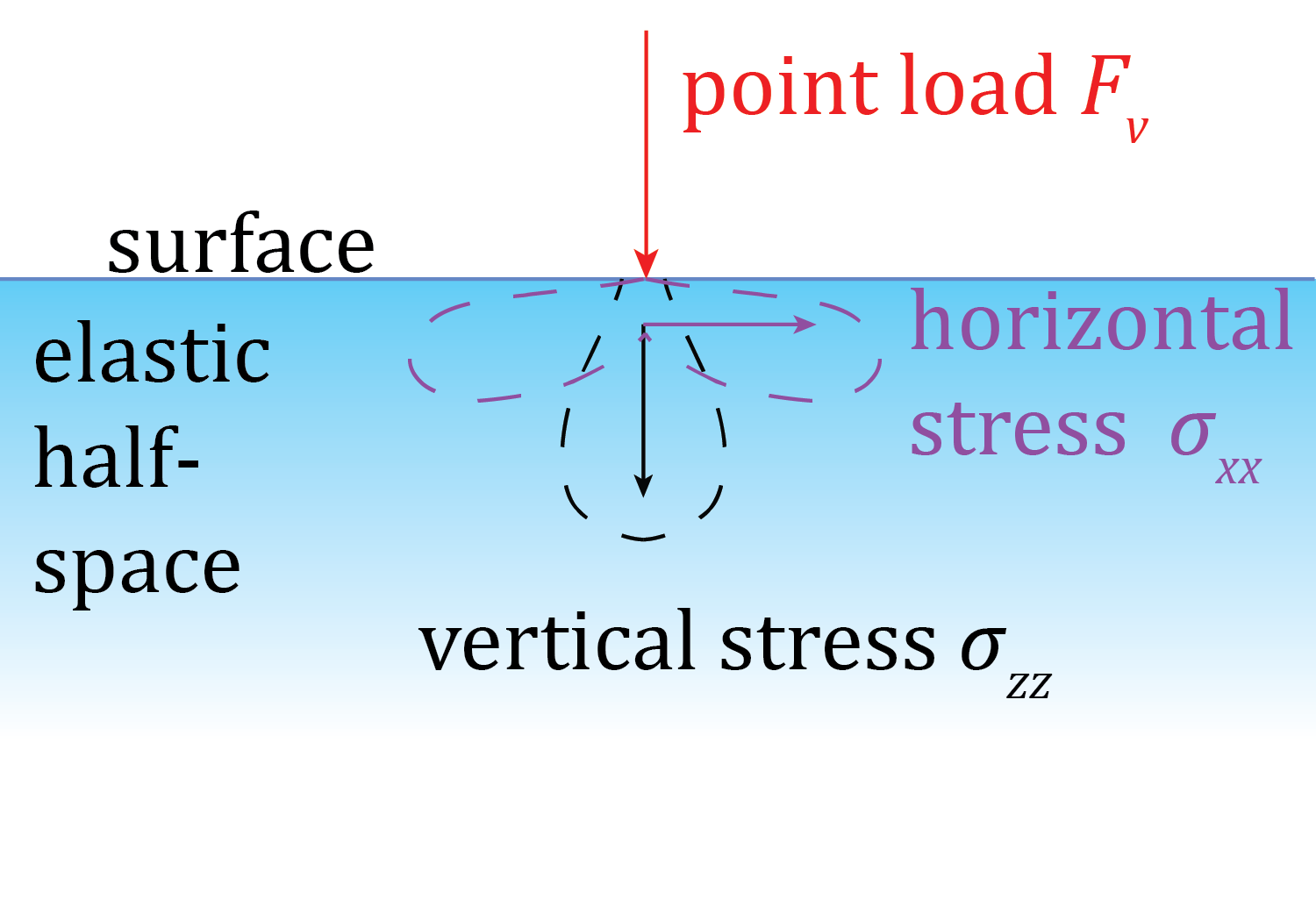 Stress components produced by a single point load
Next, we need to go from a single point load to an array of point loads. One of the nice things about small stresses and strains in elastic halfspaces is that they are addative, so the stress field from topography is basically the sum of the stresses from the individual point loads. We could go through point by point and calculate the stress field, but there is a much better way to do it. Because of the superposition principle, we can take the sort of general solution to the Boussinesq's solution above, i.e. when \(F_v=1\), and convolve this with the field of vertical forces \(F_v(x,y)\), which is the DEM times density \(\rho\) and gravitational force \(g\), yielding the stress tensor field \(M^B(x,y,z)\) (M stands for Mountain):
where \(*\) is the convolution operator.
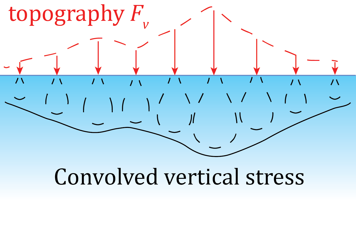 Stress componentes from an array of point loads representing topography
This calculation can be sped up tremendously (for large arrays) because of the [convolution theorem][conv_theor] which states that in cases like this, a convolution in the space domain is equivalent to a multiplication in the time domain. This means that we can take the Fourier transforms of both the Green's functions (\(G^B\)) calculated over some area, and the \(F_v\) array, and then multiply those and transform the product back, instead of doing a space-domain convolution. This is great because both the Fourier transforms and the multiplication are much faster operations than the space-domain convolution.
Next step: Horizontal topographic forces
Up to this point, the methods as described have been thought up by many scientists back to at least Harold Jeffreys. However, the result isn't quite complete. Liu and Zoback (1992) took these calculations a step further and accounted for the effects of the irregular surface above (but connected to) the halfspace into account. This includes both a correction for the horizontal shear stress induced by the effects of slope on the halfspace, and for how the irregular surface affects the propagation of stresses.
This step takes the topography and the uppermost stresses from the previous result, and yields a field of horizontal loads \(F_h(x,y)\) at the surface of the halfspace. Then, it uses Cerruti's solutions for stresses in a halfspace from a horizontal point load on the surface to propagate those stresses. The steps are exactly the same as previously, except that the process has to be done for horizontal loads in both the \(x\) and \(y\) directions. This produces a stress field \(M^C(x,y,z)\) that will be added to \(M^B(x,y,z)\) to produce the final topographic stress field \(M(x,y,z)\).
The horizontal loading functions are
and
Cerruti's solutions are as follows (assuming a point source loading in the \(+x\) direction:
These equations are then re-used, with \(x\) and \(y\) switched, to calculate the stresses from loads in the \(y\) direction.
Here is the code to do all of this:
Calculating the topographic stress field
In this section, we calculate the 3D topographic stresses in the region below the DEM. We first calculate the vertical (Boussinesq) stresses, then the horizontal/ slope (Cerruti) correction, then add them together.
from __future__ import division
import numpy as np
import halfspace.load as hs
import halfspace.sandbox as hbx
import time
import h5py
import json
Set some path and file names.
We use compressed HDF5 files for storage, using the h5py library.
stress_dir = '../stress_arrays/'
b_stress_file = stress_dir + 'baloch_bouss_stress.h5'
c_stress_file = stress_dir + 'baloch_cerr_stress.h5'
stress_file = stress_dir + 'baloch_topo_stress.h5'
dem_file = '../test_data/dem/baloch_dem_utm41n_445m.npy'
dem_metadata_file = '../test_data/dem/baloch_dem_metadata.json'

d_meta = json.load(open(dem_metadata_file, 'r')) # DEM metadata dictionary
Set up the problem
For the current implementation of halfspace (v 0.5), topography and gravity are negative, and depth is positive. Future versions of halfspace may consider topography (above sea level) and gravity as positive; this will change the coordinate system from the current left-handed system (East, North, Down) to right-handed (East, North, Up). So check the version and release notes.
rho = 2700  # density in kg m^-3
g = 9.81    # gravitational force in m s^-2
Fv = - rho * g
study_res = int(d_meta['x_res_m']) # resolution for topography, filters, etc.
z_res = 1000
b_conv_mode = 'valid'
c_conv_mode = 'same'

z_min = int(d_meta['x_res_m'])
z_max = z_min + 26000
z_len = int( (z_max - z_min) / z_res + 1)
z_vec = np.linspace(z_min, z_max, num=z_len)

kernel_rad = 1.5e5
kernel_len = int( kernel_rad * 2 / study_res +1 )
kernel_shape = np.array( [kernel_len, kernel_len] )
Load topography (DEM)
print('loading')
t0 = time.time()
topo = np.load(dem_file)
topo *= -1 # new solutions use negative topo
topo_shape = topo.shape
t1 = time.time()
print('done in', t1 - t0, 's')
Optional: pad DEM for FFT convolution
Depending on the relative sizes of the DEM, fault, and kernel width, it may be desirable to pad the DEM prior to convolution. In our case, the fault is sufficiently far from the borders of the DEM that no padding should be necessary.
pad_dem = False

if pad_dem:
    topo_prepad_shape = topo.shape
    topo = np.pad(topo, kernel_len//2, mode='constant', constant_values=[0.])
    topo_shape = topo.shape
Now for the automated part.
All the configuration should be done above this point, and below this, the cells can simply be executed.
Therefore, when using this guide as a template to do this work for different locations, you don't need to modify anything below here.
Do some configuration and make empty topo stress arrays
b_out_x, b_out_y = hbx.size_output(kernel_shape, topo_shape, mode=b_conv_mode)
b_out_size = np.array( (b_out_x, b_out_y, z_len ) )
b_stress = np.empty( (b_out_size) )

b_db = h5py.File(b_stress_file)
b_dict = {}
comp_list = ['zz', 'xy', 'xz', 'yz', 'xx', 'yy']
Boussinesq convolution
t2 = time.time()
for comp in comp_list:
    print('working on {} stresses'.format(comp) )
    b_dict[comp] = b_stress.copy()

    for i, z in enumerate(z_vec):
       b_dict[comp][:,:,i] = hs.do_b_convo(component=comp,  z=z, Fv=Fv,
                                           load=topo, load_mode='topo',
                                           conv_mode=b_conv_mode,
                                           kernel_radius=kernel_rad,
                                           kernel_res=study_res)

    b_dict[comp] *= 1e-6  # scale results to MPa

    b_db.create_dataset('b_{}_MPa'.format(comp), data = b_dict[comp],
                     chunks = True, compression = 'gzip')

    del b_dict[comp]

print('done with Boussinesq calcs in', (time.time() - t2) / 60., 'm')
Cerruti convolution
Calculate horizontal loading functions
# Boussinesq stresses for xx, xy and yy are used in the loading function
b_xx_top = b_db['b_xx_MPa'][:,:,0] * 1e6
b_xy_top = b_db['b_xy_MPa'][:,:,0] * 1e6
b_yy_top = b_db['b_yy_MPa'][:,:,0] * 1e6
b_shape = b_xx_top.shape

topo = hs._centered(topo, b_shape)

topo_dy, topo_dx = np.gradient(topo, study_res)
# make horizontal loading functions
Fht_x = topo * Fv * topo_dx
Fhb_x = b_xx_top * topo_dx + b_xy_top * topo_dy

Fht_y = topo * Fv * topo_dy
Fhb_y = b_yy_top * topo_dy + b_xy_top * topo_dx

Fh_x = Fht_x + Fhb_x
Fh_y = Fht_y + Fhb_y
# make Cerruti output arrays
c_x = np.zeros([topo.shape[0], topo.shape[1], z_len])
c_y = c_x.copy()
c_db = h5py.File(c_stress_file)
t_db = h5py.File(stress_file)

del topo # save some ram

cerr_x = {}
cerr_y = {}
total_dict = {}
Do Cerruti convolutions
t3 = time.time()
for comp in comp_list:
    print('working on {} stresses'.format(comp))

    cerr_x[comp] = c_x.copy()
    cerr_y[comp] = c_y.copy()

    for i, z in enumerate(z_vec):
        cerr_x[comp][:,:,i] = hs.do_c_convo(component=comp, f_dir='x',z=z,
                                            load=Fh_x, kernel_res=study_res,
                                            kernel_radius=kernel_rad,
                                            conv_mode=c_conv_mode) * 1e-6

        cerr_y[comp][:,:,i] = hs.do_c_convo(component=comp, f_dir='y', z=z,
                                            load=Fh_y, kernel_res=study_res,
                                            kernel_radius=kernel_rad,
                                            conv_mode=c_conv_mode) * 1e-6

    print('saving {} data'.format(comp))
    c_db.create_dataset('c_{}_x_MPa'.format(comp),
                      data = cerr_x[comp], chunks=True, compression = 'gzip')

    c_db.create_dataset('c_{}_y_MPa'.format(comp),
                      data = cerr_y[comp], chunks=True, compression = 'gzip')

    print('adding all results together')
    total_dict[comp] = (b_db['b_{}_MPa'.format(comp)][:,:,:] +  cerr_x[comp]
                        + cerr_y[comp] )

    t_db.create_dataset('{}_MPa'.format(comp), data=total_dict[comp],
                        chunks = True, compression = 'gzip')

    del total_dict[comp]
    del cerr_x[comp]
    del cerr_y[comp]

print('done with topo corrections in', (time.time() - t3) / 60., 'm')
Close HDF5 files
b_db.close()
c_db.close()
t_db.close()
print('done in', (time.time() - t0) / 60., 'm')
Done!
The files baloch_cerr_stress.h5 and baloch_bouss_stress.h5 take up a lot of room, and may be deleted, unless inspection of them is desired (and if so, it may be simpler to just generate them again, rather than keep ~3-8 GB (depending on padding) of somewhat useless data on hand).
Table of Contents for the halfspace tutorial
- Installation and configuration
- Preparing a Digital Elevation Model file
- Preparing the coseismic slip model
- Calculating the topographic stress field
- Calculating the topographic stresses on the fault
- Bayesian inversion of tectonic stress pt. 1: Rake inversion
- Bayesian inversion of tectonic stress pt. 2: Conditions at failure